NLP of WhatsApp Conversation

I’ve used the Natural Language Processing (NLP) powers of the NLTK Python library in the past. However, I feel like I’ve only brushed the surface of it’s capabilities - so, my goal here was to delve a bit deeper, and try to extract some interesting insight from some of my own textual WhatsApp data with the NLTK library.

Data comes in all shapes and sizes. However, a lot of the time it’s unstructured (or at least semi-structured). Think of the vast amount of textual documents that exist: books, emails, webpages, documents etc etc, the list is incredibly long! Around 80% of the worlds data is unstructured (according to Gartner …Google it). I could bang on for a few paragraphs about how underused textual data is to gain insight - mostly due to how difficult it’s perceived to be. Instead, to save time, I’ll post some relevant links at the end of this article.

Anyway, back to the task at hand. Firstly, I got full consent from the other person in the WhatsApp chat to play around and publish our chat data for the internet to see. However, for a bit of privacy, I’ve anonymised the data by performing a find and replace all on the names, naming us Person_1 and Person_2. Now, into the nitty gritty.

Obtaining the Data

The data used here was from a WhatsApp chat exported from my phone - clicking on the contact icon in a conversation and then selecting ‘export chat’ (without media).

The txt file has a format like so:

["[02/07/2017, 5:47:33 pm] Person_1: Hey there! This is the first message",
 "[02/07/2017, 5:48:24 pm] Person_1: This is the second message",
 "[02/07/2017, 5:48:44 pm] Person_1: Third…",
 "[02/07/2017, 8:10:52 pm] Person_2: Hey Person_1! This is the fourth message",
 "[02/07/2017, 8:14:11 pm] Person_2: Fifth …etc”]

I approached my analysis of the WhatsApp data from two different angles; one focussing on ‘core’ NLP, and the other was to make use of the datetime stamp at the beginning of every message line. To stick with the intended theme of this, however, I’ll explain the more involved NLP stuff first and then go on to explain the ‘other’ insight I leveraged, as an added bonus.

NLP - Classifying Dialogue, Lexical Diversity and Emojis

To analyse the WhatsApp data, firstly, the txt file needed to be parsed and the data formatted. This involved a few subtle steps to achieve the end-goal of creating a dictionary, constructed of two keys (one for each person in the chat) with each of the respective values a list of the persons tokenised sentences.

ppl=defaultdict(list)

for line in content:
    try:
        person = line.split(':')[2][7:]
        text = nltk.sent_tokenize(':'.join(line.split(':')[3:]))
        ppl[person].extend(text)   # If key exists (person), extend list with value (text),
                                   # if not create a new key, with value added to list
    except:
        print(line)  # in case reading a line fails, examine why
        pass

>>> ppl = {'Person_1' : ['This is message 1', 'Another message',
'Hi Person_2', ... , 'My last tokenised message in the chat'] ,
 'Person_2':['Hello Person_1!', 'How's it going?', 'Another messsage',
  ...]}

This dictionary provides the basis for the NLP insight.

Classifying Dialogue

Classifying the tokenised messages was achieved by training a Naive Bayes classifier on a training set of some pre-categorised chat-style messages - namely the nltk nps_chat corpus.

posts = nltk.corpus.nps_chat.xml_posts()

def extract_features(post):
    features = {}
    for word in nltk.word_tokenize(post):
        features['contains({})'.format(word.lower())] = True
    return features

fposts = [(extract_features(p.text), p.get('class')) for p in posts]
test_size = int(len(fposts) * 0.1)
train_set, test_set = fposts[test_size:], fposts[:test_size]
classifier = nltk.NaiveBayesClassifier.train(train_set)

The trained model could be then tested against the test set, and against some simple user input. The model was able to categorise a tokenised sentence into one of 15 different categories, such as; ‘Greet’, ‘Statement’, ‘Emphasis’, ‘Emotion’, ‘ynQuestion’, etc. to a fairly decent degree of accuracy, for example:

classifier.classify(extract_features('Hi there!'))
>>>'Greet'
classifier.classify(extract_features('Do you want to watch a film later?'))
>>>'ynQuestion'

Running the model on the WhatsApp data, counting the occurrences for each category and normalising the counts produces:

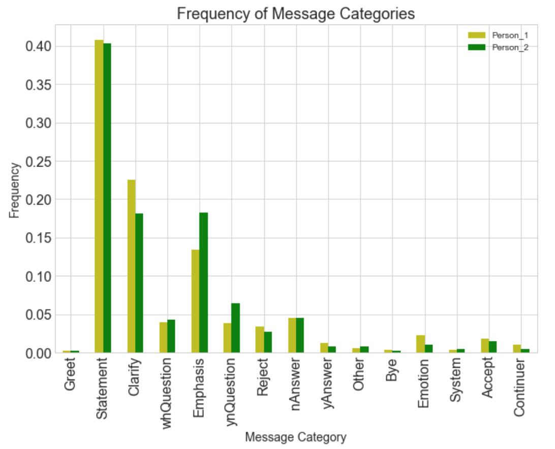
From this, we’re able to see some subtle differences in the way each person communicates, for example, Person_2 uses a lot more emphasis and asks more yes/no questions than Person_1. This could be something quite interesting to look into deeper, for example, I could try and identify a person by the way they are talking, or try and find out if a person has a specific way of messaging or is it recipient dependant? Maybe another time.

Lexical Diversity

Working out who uses the most varied set of words, i.e. who has the largest vocabulary (in the chat at least…) is fairly straightforward using each person’s list of words:

def lexical_diversity(text):
    return len(set(text)) / len(text)

for key, value in ppl.items():
    wrds=[]
    for line in ppl[key]:
        words = nltk.word_tokenize(line)
        wrds.extend(words)

    tagged = nltk.pos_tag(wrds, tagset='universal' )
    print("{}'s lexical diversity: {} \n".format(key, lexical_diversity(tagged)))

>>> "Person_1's lexical diversity: 0.14021"
>>> "Person_2's lexical diversity: 0.14322"

Disclaimer: this is only based on the chat and probably doesn’t hold precisely true in ‘real-life’. Although, it can used for bragging rights…

Emojis

Emojis are everywhere. Since being included in Apple’s 2011 IOS5 operating system they have proliferated our messages and have been likened to a language in themselves. You only have to Google something along the lines of ‘Emojis as a language’ to see for yourself the vast amount of articles written on the topic.

To handle them in this example I could’ve converted them to their unicode representation, however that would be quite boring. Instead, I used the ‘emoji’ Python library to handle them, which keeps them ‘as is’. I picked out all the emojis used by each person and counted their most used:

def extract_emojis(str):
  return ''.join(c for c in str if c in emoji.UNICODE_EMOJI)

for key, val in ppl.items():
    emojis=extract_emojis(str(ppl[key]))
    count = Counter(emojis).most_common()[:10]

    print("{}'s emojis:\n {} \n".format(key, emojis))
    print("Most common: {}\n\n".format(count))

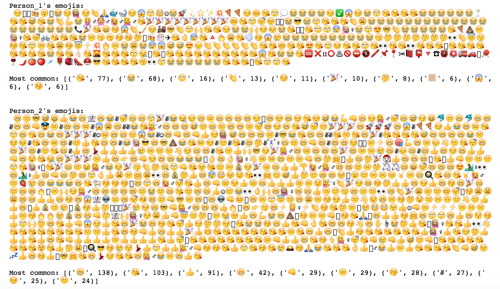
Cool! It’s quite interesting to visually see how one person uses more emojis than the other, and the difference in how each person uses them to express their emotions.

Time Series Analysis

Sentiment Against Time

Before moving completely away from NLP altogether, I’ll look at combining message sentiment with the time series component of the message. To do so, requires handling the data slightly differently than previously.

Upon parsing the file, the message has it’s sentiment calculated using the NLTK ‘Vader Sentiment Intensity Analyzer’ module. This number (a spectrum from +1 for really positive, to -1 for really negative) is added as a row to a Pandas dataframe, along with the datetime stamp of the message and the person that sent the message. The vader module is really useful in this case as it can calculate sentiment from ‘: )’ faces (but not emojis - instead I converted these to their unicode description and calculated the sentiment of this …which works quite well).

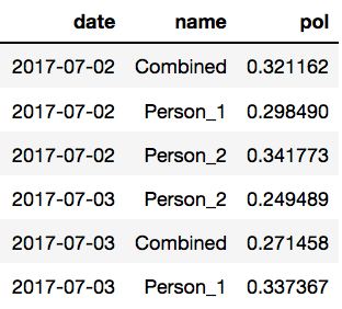
Plotting sentiment against the datetime initially turned out to be quite messy, so this process needed to be refined slightly. There are many different sentiment scores for the same day, so the first step was to calculate the mean sentiment for each day, grouping by datetime & person and taking the mean of the sentiment score. So, in the end I had a Dataframe looking a bit like this:

Even plotting the average score for each day proved messy, so my final step was to take a rolling average over 10 days, and plot the mean sentiment score for the middle of this rolling time frame.

i=0
for label, df in final.groupby('name'):
    new=df.reset_index()
    new['rol'] = new['pol'].rolling(10).mean() # rolling mean calculation on a 10 day basis
    g = new.plot(x='date', y='rol', ax=ax, label=label, color=colours[i]) # rolling mean plot
    plt.scatter(df['date'].tolist(), df['pol'], color=colours[i], alpha=0.2) # underlying scatter plot
    i+=1

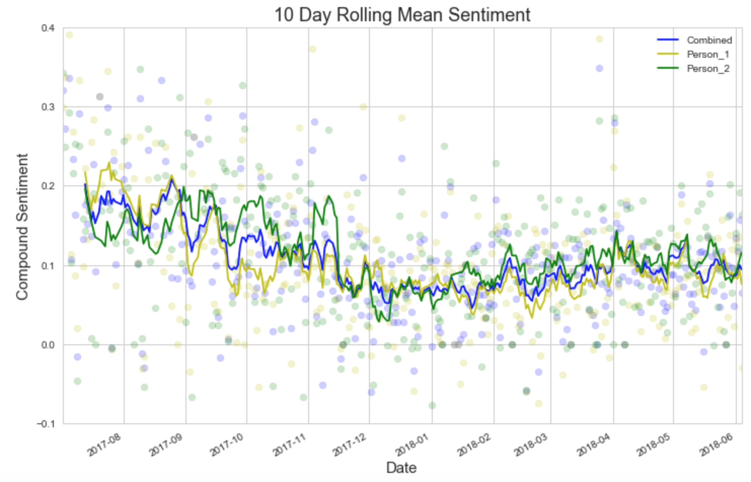
This is much better: calculating a rolling mean of the polarity makes the data a lot clearer to see what’s going on. Each person experiences periods of local highs and lows, and their sentiment ebbs and flows over time. Also, on the whole, Person_2 has had consistently, slightly higher mean sentiment from September onwards. COOL!

Frequency of Messages

As promised, here is the added bonus of time series analysis. I won’t go into too much detail how I did this, but essentially, I wanted to look at how message frequency varies by both: time of day and by day of the week. As another layer of insight, I also shaded each day with respect to their total message count.

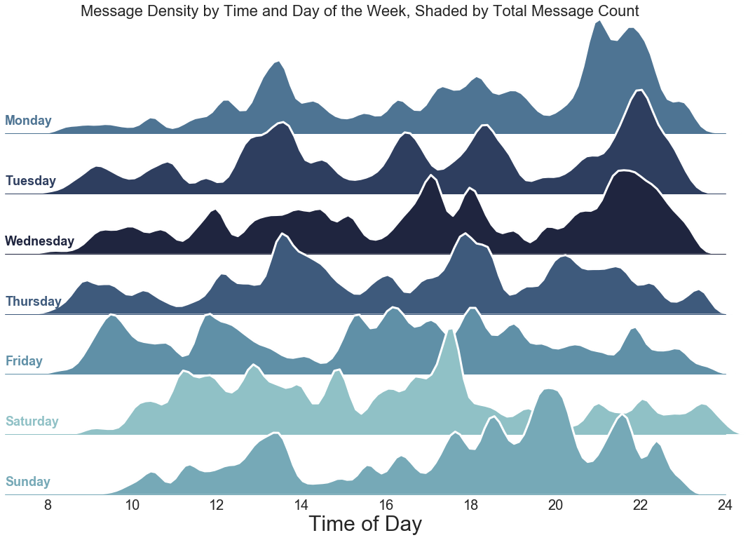
It’s quite interesting to see clear differences in message density between days of the week. Monday, Tuesday, and Wednesday follow a similar pattern with a lot of messages sent in the evening. Whereas Thursday, Friday, and Saturday have less messages sent on the whole, are spread more evenly, and with peaks in the afternoon.

Summary

Hopefully I’ve demonstrated some of the insight that can be leveraged from textual data with NLTK. As the data itself was my own, the various pieces of insight were hugely interesting for me. To this end, all my commented code is available to view here on GitHub, so you can run this with your own WhatsApp data and potentially build some more insight into this. There’s also some various other bits I haven’t written up here, such as POS tagging and creating wordclouds.

At a time of heightened public awareness about data privacy, I think one of the more empowering things you can do is try and gain insight from your own data. ✌️

Links

My NLP WhatsApp GitHub repo

NLTK Book

IBM Textual Data for Insight - Article

Article Main Banner Image, Credit: Flaticon.com