K-means Clustering FIFA 18 Player Data

K-means clustering is a method of unsupervised learning to group unlabelled data from a multi-dimensional dataset into a pre-defined number of clusters. Quite wordy that. Essentially, it’s an algorithm that works to find groups (or clusters) within a dataset - a really useful tool, with lots of potential real-world applications. Here, as a practical example, I’ll look at clustering Premier League footballers based on their FIFA 18 statistics.


The Dataset

The data I used for this is from the EA Sports game - FIFA 18. I downloaded it as a Kaggle dataset here and loaded it into a Pandas dataframe.

Some sample rows and columns of the dataset:

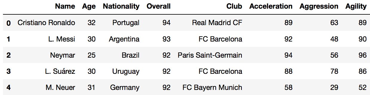
The data contains basic information on every player in the game such as; Name, Club, Nationality, and Age. More importantly, for this purpose, it contains all the physical and skill attributes; Sprint Speed, Free Kick Accuracy, Heading Accuracy etc. Also, ratings for each playing position are included - e.g. CAM, RB, GK etc.

There are numerous ways I could go about the K-means clustering, but for this, I settled on the idea of comparing players from the team I support - Newcastle United [insert pun here], against those from Manchester United. I want to compare the playing styles of the individual players, not based on their ability, so I will need to weight their stats for their respective teams. Before I can get to the stage of employing the K-means clustering, I need to first clean and then pre-process the data.

Fortunately, in this case there was only minimal cleaning required:

On closer inspection of the data, several of the columns were strings, whereas they needed to be integers. This was a quick fix:

for col in fix_cols:  # fix_cols is a list of all numeric columns

    df[col] = df[col].apply(lambda x : eval(str(x)))

Filtering the players to a new dataframe from just these two clubs:

dfnm = df[(df.Club == 'Newcastle United') | (df.Club == 'Manchester United')]

Pre-processing and PCA

Now, the data is ready to get working on and move towards clustering.

Before clustering the data, I will reduce the number of dimensions I want to base the clustering upon (namely all the skill and stat numeric columns) to two dimensions using Principal Component Analysis (PCA). To do so, the data first needs to be normalised. Usually this’d involve normalising over the entire dataset, but since I want to compare players from both teams, not based on their ability but on their playing style, I’ll normalise the players stats based on their respective team.

dfnm = dfnm.groupby('Club').transform(lambda x: (x - x.mean()) / x.std())

Now reducing the 60+ numeric dimensions, to two with PCS:

x = dfnm.values # returns a numpy array
min_max_scaler = preprocessing.MinMaxScaler()  # sklearn scaler
x_scaled = min_max_scaler.fit_transform(x)  # fit scaler
X_norm = pd.DataFrame(x_scaled)

pca = sklearnPCA(n_components=2) # 2-dimensional PCA
transformed = pd.DataFrame(pca.fit_transform(X_norm)) # new dataframe

Nice! This essentially turns a set of correlated features into a set of linearly uncorrelated ones, capturing the greatest variability between features. In a simplified view, these two dimensions don’t represent any specific attribute of the player, but instead is relative to the entire dataset.

Clustering

One major factor in K-means clustering is the number of clusters the final grouping should have. One method to determine this is via the ‘elbow method’ - plotting number of clusters against the sum of squared errors. A good number of clusters to choose is at the plot’s “elbow” - the point where adding another cluster doesn’t reduce the sum of squared errors too much. It gives a fairly good approximation but is not foolproof, so knowledge of the data helps with this too.

Mean Square Errors vs Number Of Clusters

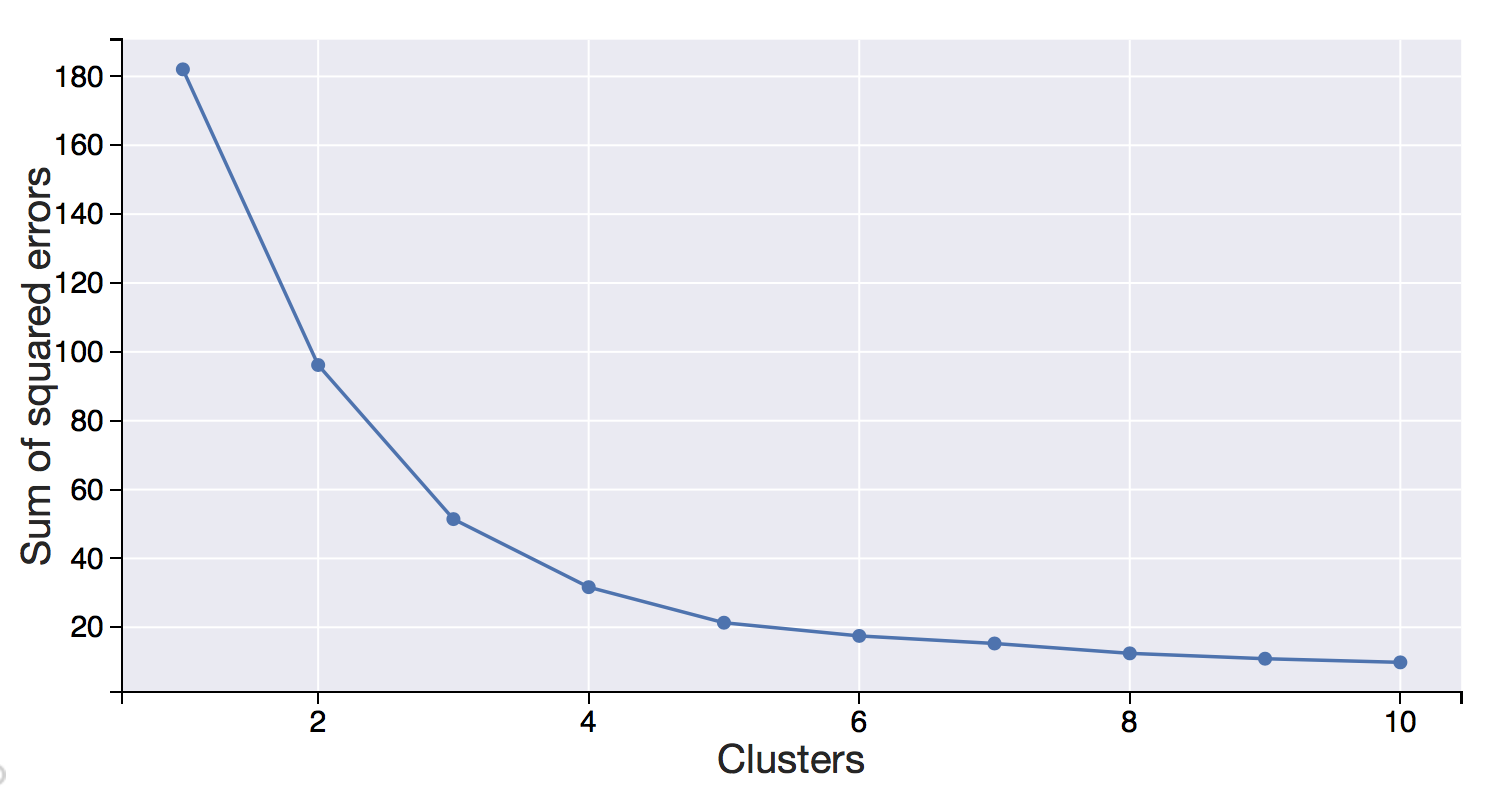
For this dataset - after a few trial-runs and from the aforementioned ‘elbow method’ - 5 clusters seem to be the most suitable fit. Employing the K-means clustering is relatively straightforward - a lot of the hard work has already been done in pre-processing the data.

kmeans = KMeans(n_clusters=5)  # Number of clusters
kmeans = kmeans.fit(transformed)  # Fitting the input data
labels = kmeans.predict(transformed)  # Getting the cluster labels
C = kmeans.cluster_centers_  # Centroid values
clusters = kmeans.labels_.tolist()  # create a list to add column to original df

Data Viz

So now we’re ready to visualise the results: plotting the two dimensions from the PCA, and colouring the groups of players from the K-means clustering:

Individual Players Two Derived Principal Components Coloured By K-means Cluster

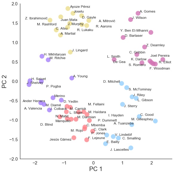
What is instantly recognisable is how well the K-means clustering algorithm has grouped type of players - Defenders in light blue (bottom-right), Defensive Midfielders and more Defenders in light Red (centre-bottom), Goalkeepers in maroon (top-right), more Attacking Midfielders in purple (centre-left), and Strikers in yellow (top-left). Mkhitaryan, Ritchie, Lingard and Young, all occupy a bit of a no-mans land, however it appears Ritchie and Mkhitaryan have a similar skillset. Also, the algorithm suggests that our answers to Paul Pogba are Henri Saivet and Jonjo Shelvey …Fairly interesting stuff.

In my notebook I’ve done another example, examining all Premier League Fullbacks, analysing their varying skill-sets. Check it out here: K-means clustering FIFA 18 data

Links

https://github.com/jcalcutt/projects/tree/master/kmeans_clustering